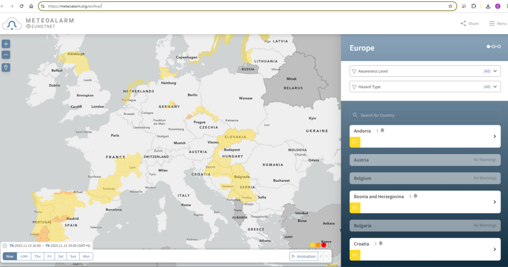
Please share research on the real-time hazard detection system………….

Latest Hyperspectral Satellite Sensors and Multi-Hazard Detection

 

The principal technological advance is not a single “all-hazard” hyperspectral sensor. It is the emergence of a satellite system of systems that combines:

• Hyperspectral infrared atmospheric sounders;
• Visible-to-shortwave-infrared imaging spectrometers;
• Ultraviolet–visible atmospheric-composition spectrometers;
• Thermal imagers;
• Passive microwave radiometers;
• Precipitation radar;
• Synthetic-aperture radar;
• Lightning imagers;
• Scatterometers, altimeters and GNSS radio occultation; and
• Ground observations, forecasting models and AI-based analytics.

Hyperspectral instruments are exceptionally good at determining what a cloud, gas, mineral, vegetation canopy, water body or surface material is made of. However, they do not directly measure every hazard. Extreme rainfall, floods, earthquakes and tsunamis require complementary radar, microwave, seismic, hydrological and ground-observation systems.

1. What makes a sensor hyperspectral?

 A conventional multispectral instrument normally observes several broad wavelength bands. A hyperspectral instrument divides the spectrum into hundreds or thousands of narrow, closely spaced channels. Each pixel therefore contains a nearly continuous spectrum: where represent location and represents wavelength. The result is a three-dimensional spectral data cube. Different materials and gases absorb or reflect radiation at distinctive wavelengths, producing identifiable spectral fingerprints. These fingerprints can reveal: Atmospheric temperature and humidity at different heights;  Water vapour transport and atmospheric instability;  Methane, carbon dioxide, ozone, sulphur dioxide and other gases;  Smoke, volcanic ash, aerosols and mineral dust;  Vegetation pigments, canopy water content and physiological stress;  Soil minerals, organic matter and moisture;  Snow grain size, dust contamination and albedo;  Burn severity and post-fire vegetation recovery;  Water quality, suspended sediment and algal pigments; and  Surface minerals associated with unstable slopes or volcanic activity.

2. Main categories of hyperspectral satellite sensors 

Sensor family	Typical observation	Principal value	Important limitation
Thermal-infrared atmospheric sounder	Thousands of IR channels, generally 4-14 km spatial resolution	Vertical temperature, humidity and trace-gas profiles; pre-convective instability	Does not directly measure surface rainfall
VSWIR surface-imaging spectrometer	Approximately 0.38–2.5 μm; typically 30–60 m pixels	Vegetation, soil, minerals, water, burn scars and gas plumes	Normally requires daylight and relatively cloud-free conditions
UV–VIS–NIR–SWIR atmospheric spectrometer	Kilometre-scale pixels	Air pollution, volcanic SO₂, ozone, aerosols, methane and carbon monoxide	Mostly column measurements; cloud and sunlight constraints
Ocean-colour hyperspectral sensor	UV, visible and near-infrared, with some SWIR bands	Phytoplankton, water quality, harmful algal blooms and aerosols	Coarser resolution and field validation requirements
Fluorescence spectrometer	Very fine bands around oxygen absorption features	Photosynthetic activity and early plant stress	Usually moderate spatial resolution and not an emergency-response sensor

3. Latest atmospheric hyperspectral sensors

FY-4C GIIRS-3 – China

FY-4C, launched on 27 December 2025, is the newest geostationary satellite carrying a hyperspectral infrared sounder. Its upgraded GIIRS instrument provides:

• Approximately 1,728 spectral channels;
• Longwave and midwave infrared coverage;
• Spectral resolution of about 0.625 cm⁻¹;
• Approximately 8 km nominal infrared resolution, with 4–8 km capability;
• Hourly coverage of a roughly 5,000 × 5,000 km regional domain; and
• Temperature, humidity, atmospheric-instability and trace-gas retrievals.

As of August 2026, FY-4C’s GIIRS, imager and lightning instruments remain under testing, while FY-4B’s GIIRS is operational at 105°E. This makes FY-4B particularly relevant to South Asia, including Bangladesh. China’s official satellite-status page and GIIRS specifications provide current details.

MTG-S1 Infrared Sounder – Europe

 MTG-S1 was launched on 1 July 2025. The satellite completed its in-orbit commissioning on 2 July 2026 and was moved to its operational position at 0° longitude. Full MTG system commissioning is planned for completion by October 2026.

Its Infrared Sounder provides: More than 1,700 thermal-infrared channels;   Longwave and midwave infrared observations; 4 × 4 km spatial resolution;  0.625 cm⁻¹ spectral resolution;  Full-disc scanning every 60 minutes;  Local-area scanning capability every 15 minutes; and  Three-dimensional temperature, humidity, wind and trace-gas information.

Its most important early-warning function is detecting moisture convergence, unstable atmospheric layers and rapid changes preceding severe convective storms. It complements the rapid imagery and lightning measurements from MTG-Imager satellites. ESA’s MTG-S1 commissioning update and Infrared Sounder specifications describe the capability.

IASI-NG on Metop-SG-A1 – Europe

 Launched on 13 August 2025, IASI-NG is the next generation of Europe’s polar-orbiting infrared atmospheric sounder. Its features include:16,921 spectral samples, compared with 8,461 on the earlier IASI;  Spectral range of approximately 3.6–15.5 μm;  0.25 cm⁻¹ spectral resolution;  Approximately 12 km individual sounding pixels;  Nearly global coverage, normally twice daily;  Improved temperature and humidity profiling near the surface; and  Detection of ozone, methane, carbon dioxide, sulphur dioxide, aerosols and dust.

It is especially valuable for numerical weather prediction, tropical-cyclone environments, heatwaves, atmospheric rivers, volcanic emissions and long-term climate monitoring. Its first spectra were received in September 2025, followed by staged calibration, validation and product release during 2026. EUMETSAT’s IASI-NG first-data report provides the current mission description.

HIRAS-II on FY-3H – China

 FY-3H was launched in September 2025 and is currently undergoing instrument testing. Its HIRAS-II provides: Approximately 3,053 channels;  Spectral coverage from about 3.92 to 15.38 μm;  0.625 cm⁻¹ spectral resolution;  14 km spatial resolution; and  A swath approximately 2,300 km wide.

It supports global temperature and humidity profiling, ozone and greenhouse-gas monitoring and numerical weather prediction. Earlier HIRAS-II instruments on FY-3E and FY-3F are already operational. Official HIRAS-II specifications give further details.

Sentinel-4 and Sentinel-5

 These are atmospheric-composition imaging spectrometers rather than broad surface-imaging systems.

• Sentinel-4, hosted on MTG-S1, observes Europe and part of North Africa every hour at about 8 km resolution. It measures nitrogen dioxide, ozone, sulphur dioxide, formaldehyde and aerosols. This supports monitoring of urban pollution, wildfire smoke, dust and volcanic emissions. ESA Sentinel-4
• Sentinel-5A, hosted on Metop-SG-A1, provides daily global coverage in seven spectral bands from ultraviolet through shortwave infrared. It targets ozone, NO₂, SO₂, formaldehyde, glyoxal, CO, methane, aerosols and UV radiation. Its product rollout follows calibration and commissioning. ESA Sentinel-5 first observations

3. Latest surface, vegetation, ocean and emissions sensors 

Mission/sensor	Important specifications	Main hazard-related applications
EnMAP	About 224 usable bands; 420–2,450 nm; 30 m pixels; 30 km swath; target revisit under four days with pointing	Drought, crop stress, soil degradation, burn severity, landslide materials, inland/coastal water quality
NASA EMIT	285 bands; 381–2,493 nm; about 7.5 nm spectral resolution; 60 m pixels; operating from the ISS through at least 2026	Mineral-dust sources, methane and CO₂ plumes, snow impurities, vegetation and hydrology
Tanager-1	Approximately 424–426 bands; about 400–2,500 nm; 30 m pixels; 18 km swath	Facility-scale methane and CO₂ emissions, vegetation, minerals and environmental contamination
PACE OCI	More than 200 hyperspectral wavelengths from UV to NIR, plus discrete SWIR bands; approximately 1.2 km; near-global coverage every 1–2 days	Harmful algal blooms, phytoplankton composition, water quality, aerosols, dust and wildfire smoke
FLEX/FLORIS	Scheduled launch 15 September 2026; 500–780 nm; 300 m pixels; 150 km swath	Direct observation of photosynthetic activity, drought and heat stress, crop and ecosystem health

EnMAP’s current technical specifications are available from DLR. EMIT’s extended mission provides 285-band data at 60 m resolution through at least 2026, according to NASA Earthdata. Tanager-1 combines a NASA-designed imaging spectrometer with a commercial satellite and has already detected facility-scale gas plumes; see NASA JPL and Tanager specifications.

PACE is currently the most advanced global polar-orbiting ocean-colour hyperspectral sensor, recording more than 200 wavelengths for phytoplankton and aquatic-hazard analysis. NASA’s 2026 PACE update describes its current performance.

FLEX is scheduled to launch in September 2026. Its FLORIS spectrometer will measure the faint fluorescence emitted during photosynthesis, providing a more direct indicator of vegetation function than conventional greenness indices. ESA FLEX mission

5. Multi-hazard detection capabilities

Hazard	Contribution from hyperspectral sensing	Essential complementary observations
Extreme precipitation and severe convection	Temperature–humidity profiles, precipitable water, instability indices, moisture convergence, cloud phase and pre-convective environment	GPM/FY-3G precipitation radar, microwave radiometers, geostationary imagery, lightning, weather radar and rain gauges
Tropical cyclones	Atmospheric thermal and moisture structure, dry-air intrusion, upper-level instability and trace-gas/aerosol environment	Scatterometer winds, microwave rain and ice, SAR, altimetry, ocean heat content and forecast models
Floods and flash floods	Daytime surface-water classification, sediment, turbidity, contamination and post-flood vegetation effects	SAR for cloud-penetrating flood extent, rainfall estimates, river gauges, DEMs and hydrological models
Drought, heat and agricultural stress	Chlorophyll, pigments, canopy water, cellulose, lignin, photosynthetic stress and soil properties	Thermal land-surface temperature, evapotranspiration, microwave soil moisture and seasonal forecasts
Wildfires	Fuel and vegetation stress, smoke composition, gas emissions, burn severity and ecological recovery	MWIR/TIR active-fire detection, geostationary rapid imagery, wind forecasts and ground fire reports
Landslides	Clay and mineral composition, vegetation stress, soil disturbance and post-event scars	Rainfall, soil moisture, DEM, Sentinel-1/NISAR InSAR deformation and ground-slope monitoring
Volcanoes	SO₂ and ash composition, thermal/mineral characteristics and hydrothermal alteration	InSAR deformation, thermal hotspots, seismicity, GNSS and ground gas measurements
Earthquakes	Post-event surface disruption and environmental damage; sometimes fault-zone mineral mapping	Seismic networks and InSAR displacement; hyperspectral imagery cannot predict earthquake occurrence
GLOFs and snow/ice hazards	Snow grain size, snow impurities, ice-albedo changes, exposed moraine and lake-water properties	SAR, optical imagery, altimetry, glacier velocity, lake-level sensors, DEMs and downstream gauges
Dust, smoke and air pollution	Mineral source composition, aerosols, NO₂, SO₂, ozone, formaldehyde, CO, methane and CO₂	Wind fields, lidar, surface air-quality stations and atmospheric-transport models
Harmful algal blooms and water pollution	Phytoplankton pigments, chlorophyll, suspended sediment, coloured dissolved material and some pollutants	Water sampling, buoys, temperature, currents and public-health thresholds
Oil spills and marine pollution	Spectral differentiation of oil, water and affected vegetation under suitable illumination	SAR for all-weather/night detection, vessel tracking and field confirmation
Tsunamis and coastal inundation	Primarily post-event inundation, sediment and ecosystem-damage assessment	Seismic networks, GNSS, deep-ocean buoys, tide gauges, radar altimetry and coastal models

 

Extreme-precipitation example

For extreme rainfall, the correct detection chain is:

1. Hyperspectral sounder: detects moisture, temperature, instability and atmospheric layers capable of supporting deep convection.
2. Geostationary imager: observes cloud growth, cloud-top cooling, overshooting tops and storm motion.
3. Lightning imager: detects rapid increases in electrical activity associated with storm intensification.
4. Microwave imager and precipitation radar: measure hydrometeors, rainfall intensity and the storm’s three-dimensional precipitation structure.
5. SAR and hydrological observations: map flooding, saturated land and affected infrastructure.
6. Forecast and impact model: combines hazard intensity with people, settlements, roads, crops and critical facilities.

NASA’s GPM Core Observatory combines a microwave imager with dual-frequency precipitation radar to measure the internal structure of storms and precipitation. It therefore measures rainfall more directly than a hyperspectral infrared sounder. NASA GPM mission

6. Recommended multi-hazard early-warning architecture

A practical national architecture should contain four observation layers:

1. Continuous geostationary layer: atmospheric profiles, rapid cloud imagery and lightning.
2. All-weather layer: SAR, microwave soil moisture, precipitation radar and scatterometer winds.
3. High-resolution environmental layer: hyperspectral, multispectral, thermal, DEM and altimetry.
4. Ground layer: weather radar, AWS, rain and river gauges, seismic/GNSS stations, air-quality monitors and community observations.

NISAR is a major new complementary capability. It entered its science phase and released provisional L-band data in July 2026. Its L- and S-band radar observations support flood mapping, soil moisture, glacier movement and centimetre-scale surface deformation associated with earthquakes, volcanoes and landslides. NASA NISAR mission

7. Priorities for Bangladesh and South Asia

For Bangladesh and neighbouring countries, the most immediately useful combination is:

• FY-4B GIIRS, AGRI and high-speed imagery from 105°E;
• FY-4C data as it completes commissioning;
• Himawari-8/9 and INSAT-3DS imagery;
• FY-3, NOAA and Metop polar atmospheric sounders;
• GPM and FY-3G precipitation measurements;
• Sentinel-1 and NISAR radar for flood, erosion, subsidence and landslide monitoring;
• Sentinel-2 and Landsat for high-resolution exposure and damage mapping;
• EnMAP, EMIT and PACE for environmental, agricultural and water-quality analysis;
• Weather radar, rainfall and river gauges for calibration and warning thresholds; and
• AI-supported data fusion linked to impact-based forecasting and Common Alerting Protocol dissemination.

The central conclusion is that hyperspectral sensing should be treated as a high-value analytical layer within a multi-sensor early-warning architecture—not as a replacement for radar, microwave, hydrological, seismic or community-based monitoring systems.

Near-term advances include FLEX in September 2026 and the planned Copernicus CHIME hyperspectral satellites, currently targeted for 2028 and 2030. CHIME is designed to provide routine 30 m hyperspectral observations across approximately 400–2,500 nm for agriculture, soils, biodiversity, water and natural-resource monitoring. Copernicus CHIME mission status

 

Extreme precipitation detection from satellites

The following analysis details the technologies, specific data products, and known limitations involved in this process.

1. The Physics of Detection: How Satellites “See” Heavy Rain

Satellites use two primary parts of the electromagnetic spectrum to detect precipitation. Understanding the difference is key to interpreting the data.

A. Passive Microwave (The “X-Ray”)

This is the most accurate method for detecting heavy rain. Raindrops and ice particles interact strongly with microwave energy.

B. Infrared (The “Cloud Top” Proxy)

Geostationary (GEO) satellites sit approx. 36,000 km above the Earth and stare continuously at the same spot.⁴

2. The “Gold Standard” Products

To solve the trade-off between LEO accuracy and GEO frequency, modern systems use constellations. They combine accurate microwave “snapshots” from LEO satellites and fill in the time gaps using GEO infrared data.

Product	Full Name	Strength for Extremes	Weakness
IMERG	Integrated Multi-sat Retrievals for GPM	The global standard. Calibrated by the GPM Core Observatory radar. Excellent for global coverage.	Tends to underestimate peak extreme intensities due to averaging (smoothing) algorithms.
GSMaP	Global Satellite Mapping of Precipitation	Often performs better in identifying orographic (mountain) heavy rain due to specific orographic correction algorithms.	Can have higher false alarm rates in some regions compared to IMERG.
CMORPH	CPC Morphing Technique	Uses microwave data primarily and “morphs” (moves) the precipitation features using wind vectors derived from GEO satellites.	struggles when microwave gaps are too long; purely morphing can miss rapid storm intensification.

3. Why Satellites Struggle with “Extreme” Events

While satellites are excellent at measuring accumulated rainfall over a month, they frequently struggle with instantaneous extreme events (e.g., flash floods).

4. Advanced Detection Techniques

To improve detection of extremes, scientists are moving beyond simple brightness temperature thresholds:

Summary Recommendation

Extreme precipitation detection from satellites

Latest Hyperspectral Sensors Enable Extreme-Precipitation Detection from Satellites

It features the newly commissioned MTG-S1 Infrared Sounder and accurately combines hyperspectral atmospheric profiling with microwave and dual-frequency radar precipitation measurements. Scientific basis: ESA MTG-S1 Infrared Sounder and NASA GPM precipitation sensors.

Hyperspectral: The New Standard in Extreme Precipitation Detection

The frontier of satellite-based precipitation detection is the transition from multispectral to hyperspectral sensing. While multispectral sensors use a few broad bands to capture images, hyperspectral sensors use hundreds of narrow, contiguous bands (see Image 5 for a detailed comparison). This “continuous spectrum” approach provides unique, high-fidelity signatures that significantly enhance the detectability of extreme events. The main breakthrough is in the use of new Hyperspectral Microwave Sounders (HyMS).

HyMS can peer through clouds, which are essential for looking at extreme convective storms. Key advantages of this new technology include:

1. Superior Sensitivity to Atmospheric Profiles: Unlike traditional sounders, HyMS can resolve fine details in the spectral signatures of water vapor, temperature, and, critically, different cloud ice types and sizes. This ability to “dissect” the vertical structure of a storm provides a direct measure of its intensity and microphysical processes, which are foundational for accurate precipitation rates (extending the capabilities of GPM, as detailed in Image 2).

2. High-Frequency LEO Constellations: The use of small-satellite and CubeSat technology (e.g., NASA TROPICS and commercial demonstrators like Spire’s HyMS) allows for the deployment of dense LEO constellations. This dramatically increases the temporal resolution making a “GPM-like” observation available much more frequently, approaching the temporal resolution of GEO satellites for detecting rapid onset, small-scale convective events.

3. Advanced Data Fusion (IMERG-Next): Integrating these high-fidelity hyperspectral datasets into the next generation of algorithms, like ‘IMERG-NEXT,‘ enables unprecedented accuracy. These systems, often using onboard AI, can combine GEO IR convective imagery (Image 1) with LEO references (Image 2) and the new high-fidelity HyMS soundings to pinpoint precipitation rates and types (e.g., distinguishing extreme rain from large hail or heavy graupel) at a sub-kilometer resolution and with a significant boost to early warning lead times (see Image 5).

Integrating Hyperspectral Data into Extreme Precipitation Systems

This detailed technical illustration acts as a definitive continuation of the data fusion narrative established in Image 3. The top section, ‘THE NEW GAME CHANGER: HYPERSPECTRAL MICROWAVE SOUNDING,‘ is a detailed diagram that contrasts a traditional ‘SINGLE BROADBAND CHANNEL’ sounder with the new ‘HUNDREDS OF NARROW CONTIGUOUS CHANNELS’ from a new ‘HYPERSPECTRAL MICROWAVE SOUNDER (HyMS) DEMONSTRATOR.‘ A spectral signature graph, ‘ATMOSPHERIC MICROWAVE EMISSIVITY,‘ illustrates how these channels uniquely resolve WATER VAPOR (H2O), OXYGEN (O2), AND CLOUD ICE SCATTERING. The bottom section shows this new data integrated into an advanced ‘IMERG-NEXT’ algorithm, which incorporates ‘ONBOARD AI’ and ‘PC-SCORE ASSIMILATION’ to produce a highly refined ‘ENHANCED EXTREME EVENT DETECTION & TYPE PINPOINTING’ product, providing detailed information on the specific precipitation type (e.g., HEAVY GRAUPEL) and an improved rain rate at a resolution that gives an additional +6 HOURS of warning lead time.

 

1) Low Earth Orbit (LEO) active radar: best for “how intense and where in the column”

Primary sensor type: Spaceborne precipitation radar

2) LEO passive microwave (PMW): best global “rain-rate signal” through clouds (but with gaps in time)

Primary sensor type: Microwave imagers/sounders used in precipitation retrieval (the workhorse for global heavy rain detection)
Examples:

Strengths for extremes: PMW is physically closer to precipitation microphysics than IR cloud-top methods; strong basis for detecting/quantifying intense rain.
Limits: revisit gaps (hours), coastal/orographic complexities, and retrieval challenges over land for certain regimes.

3) Geostationary (GEO) IR imagers: best for continuous monitoring and “rapid detection,” weaker for true intensity

Primary sensor type: Visible/IR multi-spectral imagers providing rapid-refresh cloud-top observations
Examples/products:

4) Lightning mappers: powerful proxy for convective intensification (not rain rate)

If your goal is operational extreme-rain monitoring (rather than instrument-level science), you typically use a fusion product such as:

Where ML/AI fits (if you are building an extreme-rain detector)

A common modern pattern is GEO IR (+ lightning) → calibrated against PMW/radar, using deep learning to improve detection skill and reduce false alarms; this is an active line of operational development for GOES-style precipitation retrieval enhancement.

Flash flood detection system (end-to-end design)

A flash flood detection system is operationally effective when it combines: (1) high-frequency rainfall estimation/nowcasting, (2) fast hydrologic response modeling at small-basin scale, and (3) clear, standardized warning products and dissemination. Globally, the World Meteorological Organization’s Flash Flood Guidance System (FFGS) is an established reference implementation for building national/regional capacity for flash flood warnings.

1) Core system architecture

A. Observations and rainfall estimation layer

Use the best available mix (in priority order):

Output: gridded rain rate and accumulations at multiple durations (e.g., 15/30/60/180 minutes).

B. Basin-scale hydrologic detection/forecasting layer

Two widely used operational concepts:

A concrete example is NOAA/NSSL’s FLASH system, built to improve flash flood warning specificity; it uses the CREST hydrologic model and produces high-resolution, rapidly updated hydrologic fields (soil moisture/streamflow) to support warnings.

Output: basin/stream-segment “threat” scores, exceedance probabilities, and short-fuse forecasts.

C. Impact and prioritization layer (what matters, where)

Flash flood detection becomes much more actionable when converted to impact-based outputs:

Output: ranked alert list + map of potential impacts.

D. Warning generation and dissemination layer

Adopt a standards-based alert object so the same warning can be broadcast across multiple channels (SMS, cell broadcast, apps, radio/TV crawlers, sirens, CAP feeds). The Common Alerting Protocol (CAP) is the widely used all-hazards standard for this purpose.

Output: CAP alerts with polygon/area, severity/urgency/certainty, guidance text, and validity time.

2) Detection logic (recommended “trigger stack”)

A robust flash flood detector should not rely on a single signal. A practical trigger stack is:

This mirrors how operational “guidance” systems (FFG/FFGS-style) are intended to translate rainfall into small-basin flood threat.

3) Where AI/ML improves performance (without replacing physics)

AI typically adds the most value in three modules:

A) Rainfall nowcasting (0-3 hours)

Spatiotemporal ML models improve short-lead detection of convective bursts that drive flash floods, especially when fused with radar + satellite.

B) Bias correction / data fusion

ML post-processing to:

C) Learned impact models

Supervised models that map “hazard + basin state + exposure” to likely impacts (road flooding probability, affected population), trained on historical events.

For operational credibility, keep ML “bounded” (monitor drift, enforce physical constraints where possible, and require human-in-the-loop sign-off for high-severity warnings).

4) Minimum viable vs advanced implementation

Minimum viable (works almost anywhere):

Advanced (higher skill, lower false alarms):

5) Operational essentials (often neglected)

Interagency workflow: forecaster ↔ disaster management ↔ local responders (FFGS emphasizes operational capacity-building and coordination).

Threshold governance: who sets/approves thresholds per basin and how updates happen after events

Verification: event-based scoring (POD/FAR/CSI by threshold and lead time) and post-event reviews

Redundant communications: CAP + non-digital fallbacks for high-risk communities

Model: 2

Designing an end-to-end flash flood detection system requires bridging the gap between meteorological observation (what is happening in the sky) and hydrological impact (what happens on the ground), and then successfully communicating that risk to the “last mile.”

Below is a technical architectural design for such a system, focusing on latency reduction and high-precision monitoring.

Phase 1: Multi-Sensor Data Ingestion (The “Eyes”)

Flash floods occur too quickly for any single sensor to capture perfectly. The system must ingest a “constellation” of data sources into a central Data Hub.

Data Source	Specific Technology/Product	Role in Flash Flood Detection
Satellite (Precipitation)	GPM (IMERG Early) or GSMaP_NRT	Provides the broad spatial view. Correction: Must be bias-corrected in real-time using ground gauges.
Satellite (Lightning)	GOES-GLM or MTG-LI	Critical Proxy: Lightning frequency correlates strongly with vertical updraft velocity. A sudden “lightning jump” is often the earliest precursor to the extreme rainfall rates that cause flash floods.
Ground Radar	X-Band or C-Band	If available, offers the highest resolution for calculating quantitative precipitation estimation (QPE).
IoT Sensors	Ultrasonic Level Sensors & Soil Moisture	“Ground truthing.” Soil moisture data (saturation level) determines if the ground will absorb the rain or immediately produce runoff.

Phase 2: The Processing Core (The “Brain”)

This is where the raw data is converted into actionable intelligence. This requires a High-Performance Computing (HPC) environment or a scalable Cloud Cluster.

1. The Hydrometeorological Chain

1. Nowcasting (0–6 Hours): Use Optical Flow or AI algorithms (e.g., ConvLSTM) to extrapolate current radar/satellite images 1–2 hours into the future. This is the first line of defense.
2. NWP Modeling: Run a rapid-update cycle of WRF (Weather Research and Forecasting).
   • Configuration: High resolution (1-3 km) with explicit convection (no cumulus parameterization).
   • Assimilation: Assimilate radar reflectivity and lightning data to “warm start” the model.
3. Hydrological Routing: Feed the rainfall output (QPE/QPF) into a hydrological model like WRF-Hydro or HEC-HMS.
   • Output: This calculates Streamflow (m/s) and Surface Runoff. It answers: Will the river banks overflow?

1. Impact-Based Forecasting (IBF)

Instead of warning “50mm of rain expected,” the system calculates impact.

• Overlay: Flood depth maps vs. Exposure Data (Population density, Critical Infrastructure, Agriculture).
• Trigger: If water level > threshold} AND population > 0, generate Red Alert.

Phase 3: Alert Generation & Dissemination (The “Voice”)

Speed is critical. The system must bypass congestion.

1. The Common Alerting Protocol (CAP)

The “Brain” outputs a CAP-formatted message (XML). This standard ensures all downstream systems (Sirens, TV, Mobile) understand the severity, location (polygon), and instruction.

1. Telecommunication Channels

1. Cell Broadcast (LBAS):
   • Mechanism: The Mobile Network Operator (MNO) broadcasts the message to every phone connected to cell towers within the danger polygon.
   • Advantage: Zero latency, no network congestion (uses signaling channels), works on non-smartphones. This is the gold standard for immediate life safety.
2. SMS Aggregators / SMPP:
   • Mechanism: Sends bulk SMS to registered databases (e.g., First Responders, Village Chiefs).
   • Advantage: Targeted. Can ask for confirmation.
   • Disadvantage: Slower; subject to queueing delays during storms.
3. USSD (Unstructured Supplementary Service Data):
   • Mechanism: Users dial a code (e.g., *123#) to “pull” the latest status.
   • Advantage: Works on 2G; excellent for farmers or local leaders to check river levels proactively.

System Architecture Diagram

To visualize how these components connect, here is the architectural flow:

Summary of Logic Flow

1. Detect: Satellite sees a “Lightning Jump” + Radar sees high reflectivity.
2. Predict: AI Model predicts 100mm rain in the next hour over District X.
3. Model: Hydrological model calculates that District X’s soil is saturated; Runoff will trigger a flash flood.
4. Target: GIS system identifies 5 villages in the path.
5. Warn:
   • Civil Defense: Receives CAP alert on dashboard.
   • Public: Phones in the 5 villages scream with a Cell Broadcast alert.
   • Local Leaders: Receive SMS instructing to open shelters.

Still to feed huge information……….Exploring the most robust ICT system for surface, atmospheric, and sea surface observation, real-time data acquisition, on-the-fly processing in, and displaying in MHEWS for awareness.

Flash flood Detection:

Flash floods are among the most devastating natural hazards globally, causing significant loss of life, property damage, and disruption to communities due to their rapid and unpredictable nature . Effective flash flood hazard detection systems are crucial for mitigating these impacts by providing timely warnings and facilitating rapid response actions . These systems integrate various technologies and methodologies, including hydrological models, meteorological data, remote sensing, Geographic Information Systems (GIS), and increasingly, advanced machine learning and artificial intelligence techniques 

The fundamental principle behind flood forecasting models involves the conservation of mass, partitioning precipitation into quickflow and baseflow based on infiltration-excess or saturation-excess mechanisms . Flood hazard can be quantified as a product of the physical process (hazard), the assets or people in its path (exposure), and their susceptibility to harm (vulnerability) .

Components and Methodologies of Flash Flood Detection Systems

1. Rainfall Monitoring and Prediction: Local rainstorms are the most significant factor inducing flash floods, especially in mountainous areas 16. Therefore, accurate and timely rainfall data are paramount.
   • Radar Imagery and Satellite Estimates: New-generation radars, combined with ground-truthing rain gauges, offer high-resolution and timely rainfall data for flash flood forecasting . Satellite data, such as GPM-based near-real-time precipitation estimates, are crucial for areas with data scarcity, particularly in arid regions prone to flash floods . The accuracy of satellite data can be evaluated using statistical indices and compared with ground-observed rain gauge data, leading to calibration for future predictions .

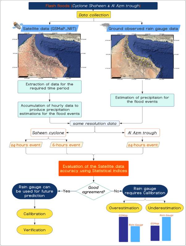
Flash floods (Cyclone Shaheen)

Source: This flowchart illustrates the process of analyzing flash floods associated with Cyclone Shaheen and the Al Azm trough, focusing on data collection, analysis, and evaluation of satellite and ground-observed data .

1. Rainfall Thresholds: Early warning systems often rely on rainfall thresholds, which can be determined using empirical methods (based on historical data), hydrological methods (considering watershed characteristics), and machine learning approaches 19. Empirical methods identify patterns between rainfall and floods but may struggle with spatial and temporal variations, while hydrological methods, though more accurate, require detailed data .
2. Rainfall Pattern Identification: A dynamic warning model for flash floods can be improved by identifying rainfall patterns, addressing the randomness and uncertainty of rainfall events .
3. Hydrological Modeling: Hydrological models simulate the movement of water across a landscape and are essential for predicting flash floods. These models can range from conceptual, often lumped and parsimonious, to process-based, distributed, and physics-rich .
   • Runoff Generation and Routing: Models aim to correctly partition precipitation into quickflow and baseflow and route the resulting water to the outlet . Infiltration models, from empirical formulas like Horton’s to complex Richards equations, are critical for representing the vertical flux of water into the soil .
   • GIS-based Hydrological Models: Geographic Information Systems (GIS) technology is extensively used in flash flood risk management for monitoring, analysis, and prediction 10. GIS-based morphometric analysis, utilizing geological, geomorphological, and hydrogeological characteristics, helps in mapping flood hazard degrees and susceptibility in arid regions . Software like the Watershed Modeling System (WMS) is also employed for flash flood simulation .
   • Urban Flood Prediction: In urban areas, models like the Storm Water Management Model (SWMM) are used to estimate road user delay and assess flood risks based on rainfall scenarios, considering both occurrence probability and economic consequences . Interpretable machine learning models, which incorporate intertwined land and built-environment features, can identify urban flash flood hotspots more efficiently than computationally expensive rainfall-runoff or hydrologic models .

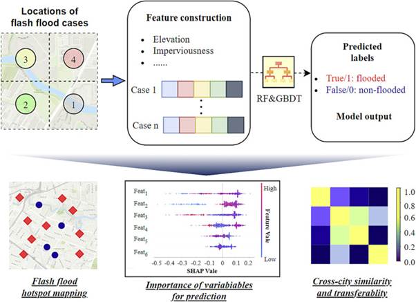
Flash-flood analysis and prediction

Source: 15 This figure depicts a comprehensive workflow for flash flood analysis and prediction, involving flash flood case locations, feature construction (e.g., Elevation, Imperviousness), machine learning models (RF&GBDT), prediction of flooded/non-flooded labels, hotspot mapping, and analysis of variable importance using SHAP values, and cross-city similarity for model transferability .

3. Sensor Networks and Real-time Data Collection: Real-time data from sensor networks is crucial for effective flash flood detection and early warning.
   • Low-Cost Sensor Systems: Prototypes using Raspberry Pi cameras can detect rising water levels and identify flash floods in real-time, even under varying environmental conditions 5. Low-cost systems utilizing Arduino boards and echolocation for water level measurement, with data transmission via mobile networks, have also been developed .
   • Ultrasonic and Infrared Sensors: Urban flash flood detection systems can employ ultrasonic and infrared sensors to provide critical information on flood type, location, and severity, which is vital given the short timescales of urban flash floods .
   • IoT Integration: The integration of IoT sensors with machine learning algorithms facilitates early flash flood detection by continuously analyzing crucial environmental variables 9. This technology aims to improve public safety by issuing early and accurate warnings .
   • Infrasound Detection: Infrasound signals from water discharges at hydroelectric dams have shown a 79% detection rate for significant water level increases downstream over a 14-year period (2008–2021) 26. This method can provide timely warnings for unexpected discharge events .
4. Artificial Intelligence and Machine Learning: AI and ML techniques are increasingly being applied to overcome challenges associated with complex hydrological processes and the need for real-time data interpretation in flash flood prediction .
   • Deep Learning Models: Convolutional Neural Networks (CNNs), including Deep 1D-CNN, are used for spatially predicting flash floods by integrating various geospatial data such as geology, soil type, land use, elevation, slope, and rainfall . These models can learn complex relationships between environmental factors and flash flood susceptibility.

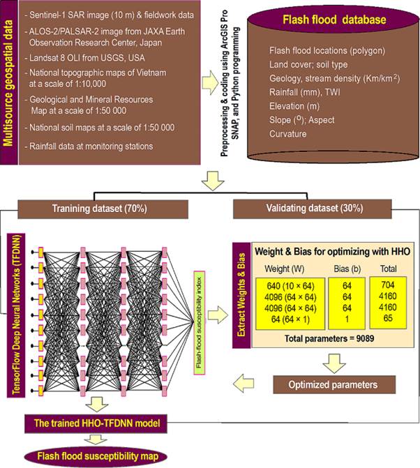
Flash-flood susceptibility map

This workflow illustrates the creation of a flash-flood susceptibility map using multi-source geospatial data, deep neural networks (TFDNN), and Harris Hawks Optimization (HHO) for weight and bias optimization .

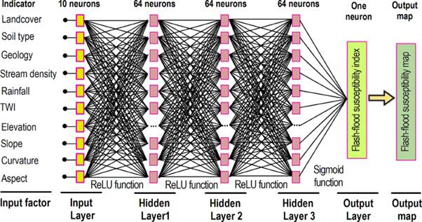
Neural network architecture fo…

 This image depicts a neural network architecture with an input layer of 10 neurons representing environmental factors (e.g., landcover, soil type, rainfall, TWI, elevation, slope, curvature, aspect), three hidden layers with neurons each using ReLU activation, and a single-neuron output layer with a Sigmoid function to generate a flash-flood susceptibility index .

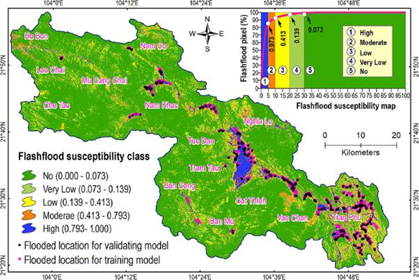
Flash-flood Susceptibility Map

This flash-flood susceptibility map uses color coding to indicate different levels of susceptibility from “No” to “High”, with pink dots marking flooded locations used for training and black dots for validating the model . An attention mechanism, specifically the convolutional block attention module (CBAM), can enhance CNN models for flash flood susceptibility mapping, addressing issues like gradient explosion and overfitting .

4. : The YOLOv8 model, a deep learning-based object detection method, can be used for real-time flash flood detection from visual data, demonstrating high confidence scores (e.g., 0.86 and 0.85) in identifying flash flood events in video feeds 29.

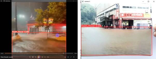
Flash flood detection using YO…

This figure shows the YOLOv8 model detecting “flash_flood” with high confidence scores in two different video feeds, indicating its application in real-time monitoring .

4. Hybrid Machine Learning Models: Novel hybrid ML models, like those combining Artificial Bee Colony (ABC) algorithms with Deep Neural Networks (DNN) and Levenberg-Marquardt (LM) algorithms, are being developed for flood subsidence susceptibility mapping 14. These models utilize historical flood data, remote sensing imagery, and various flood conditioning factors to produce flood susceptibility maps with accuracy evaluations .

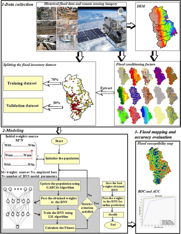
Flood Susceptibility Mapping

 This flowchart outlines the process of flood susceptibility mapping and analysis, covering data collection, modeling using a hybrid ABC-DNN-LM approach, and flood mapping with accuracy evaluation using ROC and AUC curves .

5. Remote Sensing and Geographic Information Systems (GIS): Remote sensing provides extensive data over large areas, essential for hazard detection and mapping. SAR (Synthetic Aperture Radar) is a valuable tool for flood inundation mapping due to its ability to penetrate clouds and darkness .
   • SAR Time Series Analysis: SAR systems detect floods by observing low radar backscatter from smooth water surfaces, which appear dark. In contrast, rougher land surfaces appear brighter . Time series analysis enables robust flood detection by identifying anomalous changes in backscatter relative to a stable baseline of normal conditions . This method can differentiate temporary floods from permanent water bodies .
   • NDWI and MNDWI: Normalized Difference Water Index (NDWI) and Modified Normalized Difference Water Index (MNDWI) distinguish water bodies based on their reflectance properties . MNDWI often outperforms NDWI, especially in urban areas, by better suppressing signals from built-up land, thus reducing false positives . These indices are foundational for rapid flood mapping .
   • Integration with DEMs: Fusing SAR data with Digital Elevation Models (DEMs) and hydraulic principles helps in creating physically realistic flood maps and estimating water levels . A pixel is considered inundated only if its elevation is below the estimated water surface elevation and it is continuously connected to a known water source .
   • Sentinel-2 Data: The Robust Satellite Technique (RST-FLOOD) has been extended to Sentinel-2 data for mapping flooded areas, providing timely and accurate information on location and extent of affected areas, which is crucial for recovery efforts .

Challenges and Future Directions Despite advancements, challenges remain in flash flood detection. These include the short lead times associated with flash floods, which make accurate forecasting difficult, and the need for more holistic analyses of model uncertainties . Non-identifiability of spatially distributed environmental models further complicates the process .

Future research aims to enhance the integration of multidisciplinary approaches, including artificial intelligence, IoT, and cloud computing, for more robust flash flood early warning and susceptibility prediction systems . This also includes improving model interpretability to facilitate trust and understanding among stakeholders . Furthermore, an objective framework for bivariate risk analysis of flash floods under the compound effect of rainfall characteristics is being developed, aiming to classify flash flood events based on intensity and process using clustering methods 34. The use of agent-based models to simulate human responses to flash flood warnings and improve evacuation performance is also an important area of study 

Designing an end-to-end flash flood detection system requires bridging the gap between meteorological observation (what is happening in the sky) and hydrological impact (what happens on the ground), and then successfully communicating that risk to the “last mile.”

………………………………………………………………………………………………………………………

References ;

• Driving Force Exploration for Flash Flood Based on Mann–Kendall Test and Geographical Detector: A Case Study of Hainan Island, China
• A global sensitivity analysis approach for identifying critical sources of uncertainty in non-identifiable, spatially distributed environmental models: A holistic analysis applied to SWAT for input datasets and model parameters
• A Flash Flood Categorization System Using Scene-Text Recognition
• 2018 IEEE International Conference on Smart Computing (SMARTCOMP)
• Enhancing community resilience in arid regions: A smart framework for flash flood risk assessment
• An agent-based model to simulate human responses to flash flood warnings for improving evacuation performance
• Water, Vol. 16, Pages 3634: Characteristics and Comparative Assessment of Flash Flood Hazard Evaluation Techniques: Insights from Wadi Haily Basin, Eastern Red Sea Coast, Saudi Arabia